The simplest SCA analysis ever

This example shows the full process to perform a complete SCA analysis and detect protein sectors from data importation, MSA filtering.

import cocoatree.datasets as c_data
import cocoatree
import matplotlib.pyplot as plt

Load the dataset

We start by importing the dataset. In this case, we can directly load the S1 serine protease dataset provided in cocoatree. To work on your on dataset, you can use the cocoatree.io.load_msa function.

serine_dataset = c_data.load_S1A_serine_proteases()
loaded_seqs = serine_dataset["alignment"]
loaded_seqs_id = serine_dataset["sequence_ids"]
n_loaded_pos, n_loaded_seqs = len(loaded_seqs[0]), len(loaded_seqs)

Compute the SCA analysis

coevol_matrix, results = cocoatree.perform_sca(
    loaded_seqs_id, loaded_seqs, n_components=3)
print(results.head())

computing weight of seq 1/1376
computing weight of seq 101/1376
computing weight of seq 201/1376
computing weight of seq 301/1376
computing weight of seq 401/1376
computing weight of seq 501/1376
computing weight of seq 601/1376
computing weight of seq 701/1376
computing weight of seq 801/1376
computing weight of seq 901/1376
computing weight of seq 1001/1376
computing weight of seq 1101/1376
computing weight of seq 1201/1376
computing weight of seq 1301/1376
   original_msa_pos  filtered_msa_pos  PC1  IC1  ...  sector_2  PC3  IC3  sector_3
0                 0               NaN  NaN  NaN  ...     False  NaN  NaN     False
1                 1               NaN  NaN  NaN  ...     False  NaN  NaN     False
2                 2               NaN  NaN  NaN  ...     False  NaN  NaN     False
3                 3               NaN  NaN  NaN  ...     False  NaN  NaN     False
4                 4               NaN  NaN  NaN  ...     False  NaN  NaN     False

[5 rows x 11 columns]

Select the position of the first sector in the results dataframe.

print(results.loc[results["sector_1"]].head())

     original_msa_pos  filtered_msa_pos       PC1  ...       PC3       IC3  sector_3
130               130              23.0 -0.090217  ...  0.029506  0.045516     False
133               133              26.0 -0.116480  ...  0.044673  0.059013     False
214               214              35.0 -0.106719  ... -0.087057 -0.046816     False
246               246              48.0 -0.130522  ... -0.028971 -0.038197     False
247               247              49.0 -0.110328  ...  0.038413  0.023443     False

[5 rows x 11 columns]

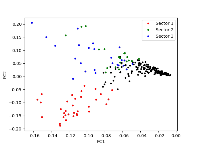
Visualizing the sectors on the first and second PC

# Plotting all elements in components
fig, ax = plt.subplots()
ax.plot(results.loc[:, "PC1"],
        results.loc[:, "PC2"],
        ".", c="black")

# Plotting elements in sectors
for isec, color in zip([1, 2, 3], ['r', 'g', 'b']):
    ax.plot(results.loc[results["sector_%d" % isec], "PC1"],
            results.loc[results["sector_%d" % isec], "PC2"],
            ".", c=color, label="Sector %d" % isec)

ax.set_xlabel("PC1")
ax.set_ylabel("PC2")

ax.legend()

<matplotlib.legend.Legend object at 0x7f90eaae3b50>

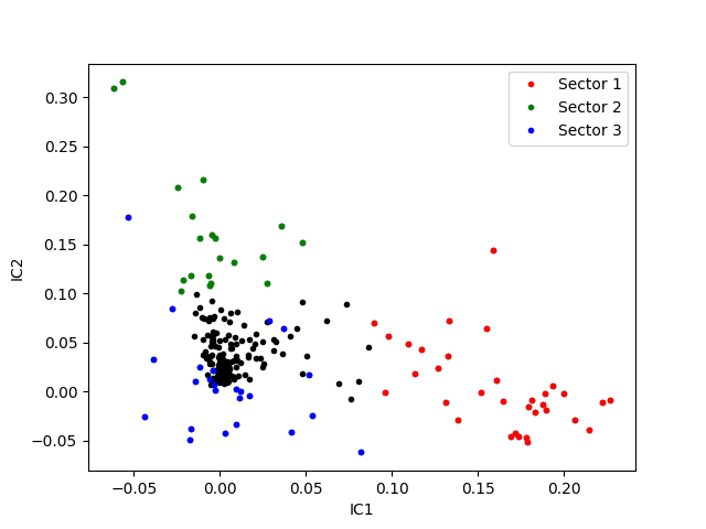
Visualizing the sectors on the first and second IC

# Plotting all elements in components
fig, ax = plt.subplots()
ax.plot(results.loc[:, "IC1"],
        results.loc[:, "IC2"],
        ".", c="black")

# Plotting elements in sectors
for isec, color in zip([1, 2, 3], ['r', 'g', 'b']):
    ax.plot(results.loc[results["sector_%d" % isec], "IC1"],
            results.loc[results["sector_%d" % isec], "IC2"],
            ".", c=color, label="Sector %d" % isec)

ax.set_xlabel("IC1")
ax.set_ylabel("IC2")

ax.legend()

<matplotlib.legend.Legend object at 0x7f90eaae3890>