A minimal coevo analysis using cocoatree.perform_sca()

This example generates the same result as A minimal coevo analysis, but uses the cocoatree.perform_sca() function, which filters sequences and returns the coevolution matrix and its associated objects of interest (PCs, ICs, XCoRs) in Pandas format.

# Author: Margaux Jullien <margaux.jullien@univ-grenoble-alpes.fr>
#         Nelle Varoquaux <nelle.varoquaux@univ-grenoble-alpes.fr>
#         Ivan Junier <ivan.junier@univ-grenoble-alpes.fr>
# License: TBD

Necessary imports

import numpy as np
import matplotlib.pyplot as plt

import cocoatree
import cocoatree.datasets as c_data
import cocoatree.deconvolution as c_deconv

Loading the dataset

serine_dataset = c_data.load_S1A_serine_proteases()
loaded_seqs = serine_dataset["alignment"]
loaded_seqs_id = serine_dataset["sequence_ids"]
n_loaded_pos, n_loaded_seqs = len(loaded_seqs[0]), len(loaded_seqs)

Performing a SCA analysis

SCA_matrix, SCA_matrix_ngm, df = cocoatree.perform_sca(
    loaded_seqs_id, loaded_seqs, n_components=3)

print('The cocoatree.perform_sca returns the following columns:')
print(df.columns.values)

The cocoatree.perform_sca returns the following columns:
['original_msa_pos' 'filtered_msa_pos' 'PC1' 'IC1' 'xcor_1' 'PC2' 'IC2'
 'xcor_2' 'PC3' 'IC3' 'xcor_3']

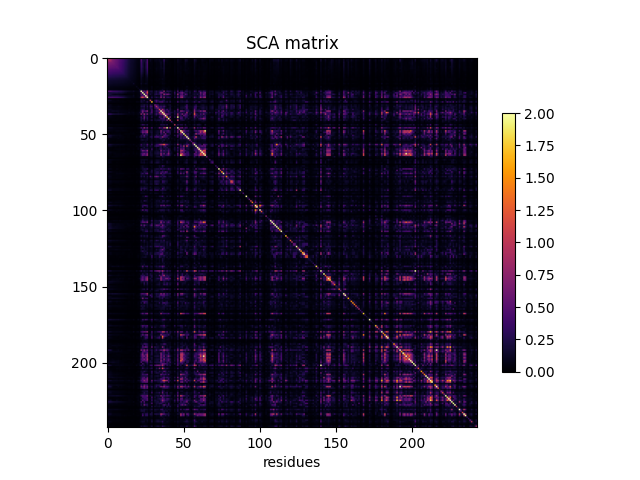
Plotting the SCA matrix

fig, ax = plt.subplots()
im = ax.imshow(SCA_matrix, vmin=0, vmax=2, cmap='inferno')

ax.set_xlabel('residues', fontsize=10)
ax.set_ylabel(None)
ax.set_title('SCA matrix')
fig.colorbar(im, shrink=0.7)

<matplotlib.colorbar.Colorbar object at 0x7f5e7194dd90>

Extracting XCoRs

n_xcors = 3
xcors = []
for ixcor in range(1, n_xcors+1):
    print('XCoR_%d:' % ixcor, end=' ')
    # extacting the unsorted xcor
    xcor = df.loc[df['xcor_%d' % ixcor]]['filtered_msa_pos'].values

    # sorting xcor according to its ICA value (from largest to smallest)
    xcor = sorted(xcor, key=lambda x:
                  -float(df.loc[df['filtered_msa_pos'] == x]
                         ['IC%d' % ixcor].iloc[0]))

    xcors.append(xcor)
    print(xcors[-1])

XCoR_1: [np.int64(64), np.int64(48), np.int64(63), np.int64(195), np.int64(182), np.int64(168), np.int64(197), np.int64(199), np.int64(108), np.int64(61), np.int64(144), np.int64(146), np.int64(198), np.int64(196), np.int64(216), np.int64(49), np.int64(192), np.int64(194), np.int64(222), np.int64(234), np.int64(145), np.int64(208), np.int64(211), np.int64(35), np.int64(235), np.int64(26), np.int64(62), np.int64(50), np.int64(155), np.int64(200), np.int64(97), np.int64(23), np.int64(73)]
XCoR_2: [np.int64(140), np.int64(202), np.int64(52), np.int64(57), np.int64(110), np.int64(111), np.int64(129), np.int64(78), np.int64(87), np.int64(58), np.int64(226), np.int64(75), np.int64(124), np.int64(128), np.int64(81), np.int64(34), np.int64(231), np.int64(32), np.int64(33), np.int64(204)]
XCoR_3: [np.int64(212), np.int64(225), np.int64(190), np.int64(180), np.int64(223), np.int64(183), np.int64(213), np.int64(210), np.int64(193), np.int64(224), np.int64(220), np.int64(172), np.int64(184), np.int64(176), np.int64(36), np.int64(217), np.int64(161), np.int64(37), np.int64(142), np.int64(160), np.int64(177), np.int64(46), np.int64(188), np.int64(24)]

A plotting function

def plot_coevo_according2xcors(coevo_matrix, xcors=[], vmin=0, vmax=1e6):
    """ A plotting function returning a reduced coevo matrix, keeping
    only XCoRs and sorting the residues according to them
    """

    fig, ax = plt.subplots(tight_layout=True)

    xcor_sizes = [len(x) for x in xcors]
    cumul_sizes = sum(xcor_sizes)
    sorted_pos = [p for xcor in xcors for p in xcor]

    im = ax.imshow(coevo_matrix[np.ix_(sorted_pos, sorted_pos)],
                   vmin=vmin, vmax=vmax,
                   interpolation='none', aspect='equal',
                   extent=[0, cumul_sizes, cumul_sizes, 0],
                   cmap='inferno')
    cb = fig.colorbar(im)
    cb.set_label("coevolution level")

    line_index = 0
    for i in range(n_xcors):
        ax.plot([line_index + xcor_sizes[i], line_index + xcor_sizes[i]],
                [0, cumul_sizes], 'w', linewidth=2)
        ax.plot([0, cumul_sizes],
                [line_index + xcor_sizes[i], line_index + xcor_sizes[i]],
                'w', linewidth=2)
        line_index += xcor_sizes[i]

    ticks = []
    for ix in range(len(xcors)):
        shift = np.sum([len(xcors[j]) for j in range(ix)])
        ticks.append(shift+len(xcors[ix])/2)

    ax.set_xticks(ticks)
    ax.set_xticklabels(['XCoR_%d' % ix for ix in range(1, len(xcors)+1)])
    ax.set_yticks(ticks)
    ax.set_yticklabels(['XCoR_%d' % ix for ix in range(1, len(xcors)+1)],
                       rotation=90, va='center')

    return fig, ax

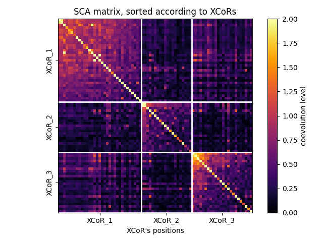
Plotting the SCA matrix according to the XCoRs

fig, ax = plot_coevo_according2xcors(SCA_matrix, xcors, vmin=0, vmax=2)
ax.set_title('SCA matrix, sorted according to XCoRs')
ax.set_xlabel('XCoR\'s positions', fontsize=10)

Text(0.5, 29.000000000000014, "XCoR's positions")

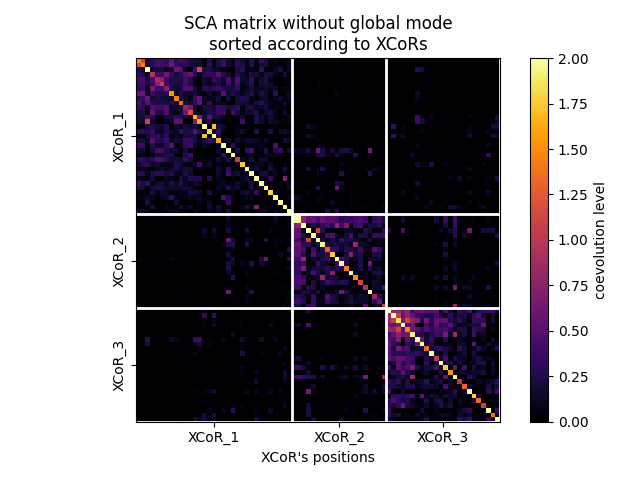
Removing a global mode (ngm = no global mode), i.e., setting largest eigeinvalue to zero

SCA_matrix_ngm = c_deconv.remove_global_correlations(SCA_matrix)

Plotting the SCA matrix without global mode according to the XCoRs

fig, ax = plot_coevo_according2xcors(SCA_matrix_ngm, xcors, vmin=0, vmax=2)
ax.set_title('SCA matrix without global mode\nsorted according to XCoRs')
ax.set_xlabel('XCoR\'s positions', fontsize=10)

Text(0.5, 29.000000000000014, "XCoR's positions")

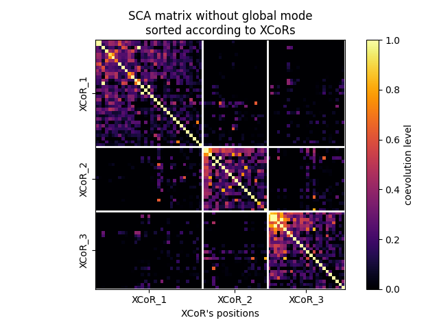
Adapting the coevolution scale

fig, ax = plot_coevo_according2xcors(SCA_matrix_ngm, xcors, vmin=0, vmax=1)
ax.set_title('SCA matrix without global mode\nsorted according to XCoRs')
ax.set_xlabel('XCoR\'s positions', fontsize=10)

Text(0.5, 29.000000000000014, "XCoR's positions")

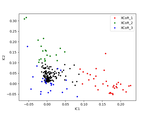
Visualizing XCoRs on independent components

# plotting IC_1 values versus IC_2 values
fig, ax = plt.subplots()
ax.plot(df.loc[:, 'IC1'], df.loc[:, 'IC2'], '.k')

# highlighting XCoR-associated values using a color code
# red: XCoR_1, green: XCoR_2, blue: XCoR_3
for xcor, color in zip([1, 2, 3], ['r', 'g', 'b']):
    ax.plot(df.loc[df['xcor_%d' % xcor], 'IC1'],
            df.loc[df['xcor_%d' % xcor], 'IC2'],
            '.', c=color, label='XCoR_%d' % xcor)

ax.set_xlabel('IC1')
ax.set_ylabel('IC2')

ax.legend()

<matplotlib.legend.Legend object at 0x7f5e71ccd910>