Mutual information versus SCA co-evolution metrics

In this example, we are comparing the results of the co-evolution analysis on serine proteases using SCA and the mutual information.

Necessary imports

from cocoatree.datasets import load_S1A_serine_proteases
from cocoatree.msa import filter_sequences

from cocoatree.statistics.position import compute_conservation
from cocoatree.statistics.pairwise import compute_sca_matrix
from cocoatree.statistics.pairwise import compute_mutual_information_matrix

import matplotlib.pyplot as plt

import numpy as np

Load the dataset

We start by importing the dataset.

For more details on the S1A serine proteases dataset, go to S1A serine proteases.

serine_dataset = load_S1A_serine_proteases()
seq_id = serine_dataset["sequence_ids"]
sequences = serine_dataset["alignment"]
n_pos, n_seq = len(sequences[0]), len(sequences)

Filtering of the multiple sequence alignment

We filter and clean the MSA

seq_kept, seq_id_kept, pos_kept = filter_sequences(sequences, seq_id)

Compute the SCA matrix

SCA_matrix = compute_sca_matrix(seq_kept)

Compute MI matrices

normalized_MI = compute_mutual_information_matrix(seq_kept)
MI = compute_mutual_information_matrix(seq_kept, normalize=False)

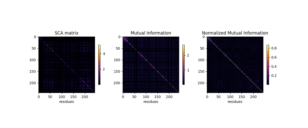
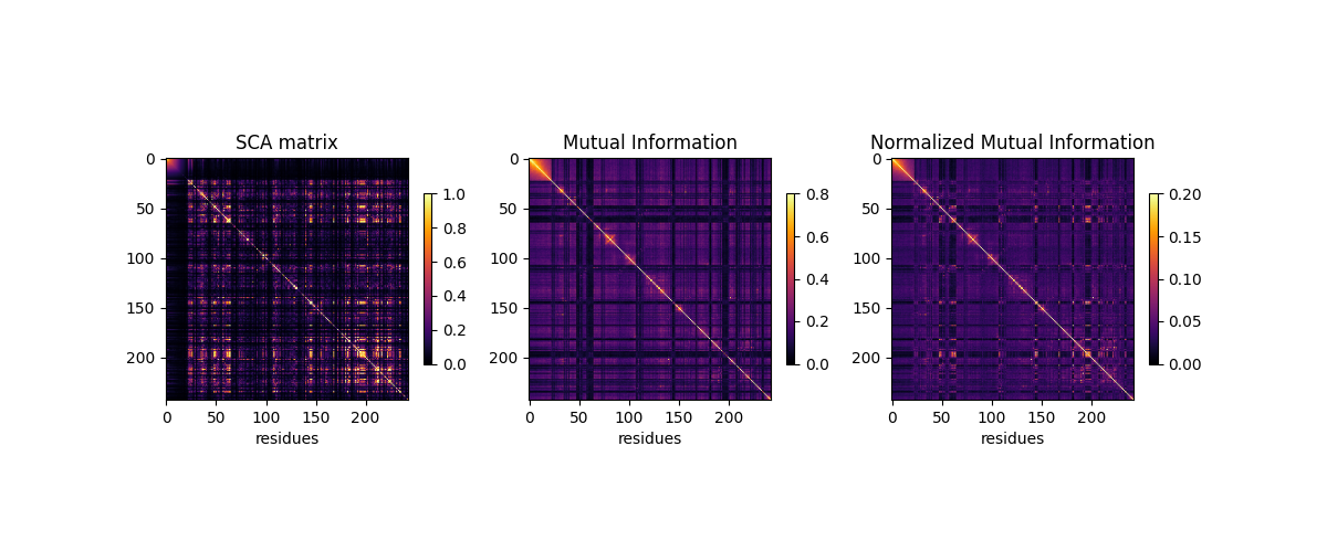
Compare MI versus SCA

The heatmap scales are adjusted to make the information visible

plt.figure(figsize=(12, 5))

for ih, (heatmap, title, vmm) in \
    enumerate(zip([SCA_matrix, MI, normalized_MI],
                  ['SCA', 'Mutual Information',
                   'Normalized Mutual Information'],
                  [[0, 1], [0, 0.8], [0, 0.2]])):
    plt.subplot(1, 3, ih+1)
    plt.imshow(heatmap, vmin=vmm[0], vmax=vmm[1], cmap='inferno')
    plt.xlabel('residues', fontsize=10)
    plt.ylabel(None)
    plt.title('%s' % title)
    plt.colorbar(shrink=0.4)

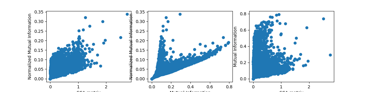
Relationships between SCA and MI’s

plt.figure(figsize=(12, 3))
plt.subplot(1, 3, 1)
plt.plot(np.triu(SCA_matrix, 1).flatten(),
         np.triu(normalized_MI, 1).flatten(), 'o')
plt.xlabel('SCA')
plt.ylabel('Normalized Mutual Information')

plt.subplot(1, 3, 2)
plt.plot(np.triu(MI, 1).flatten(), np.triu(normalized_MI, 1).flatten(), 'o')
plt.xlabel('Mutual Information')
plt.ylabel('Normalized Mutual Information')

plt.subplot(1, 3, 3)
plt.plot(np.triu(SCA_matrix, 1).flatten(), np.triu(MI, 1).flatten(), 'o')
plt.xlabel('SCA')
plt.ylabel('Mutual Information')

Text(769.1928104575164, 0.5, 'Mutual Information')

Relationship between coevolution metrics and conservation

plt.figure(figsize=(12, 3))

Di = compute_conservation(seq_kept)

for ih, (heatmap, title) in enumerate(zip([SCA_matrix, MI, normalized_MI],
                                          ['SCA', 'MI', 'normalized MI'])):
    plt.subplot(1, 3, ih + 1)
    cumul = np.sum(heatmap, axis=0) - np.diag(heatmap)
    plt.plot(Di, cumul, 'o')
    plt.xlabel('conservation')
    if ih == 0:
        plt.ylabel('cumulative score')
    plt.title(title)