Perform full SCA analysis on the S1A serine protease dataset

This example shows the full process to perform a complete SCA analysis and detect protein sectors from data importation, MSA filtering.

Finally, we export a fasta file of the residues contributing to the first sector.

# Author: Margaux Jullien <margaux.jullien@univ-grenoble-alpes.fr>
#         Nelle Varoquaux <nelle.varoquaux@univ-grenoble-alpes.fr>
#         Ivan Junier <ivan.junier@univ-grenoble-alpes.fr>
# License: TBD

Import necessary

import cocoatree.datasets as c_data
import cocoatree.io as c_io
import cocoatree.msa as c_msa
import cocoatree.statistics.position as c_pos
import cocoatree.statistics.pairwise as c_pw
import cocoatree.deconvolution as c_deconv

import matplotlib.pyplot as plt
import numpy as np

Load the dataset

We start by importing the dataset. In this case, we can directly load the S1 serine protease dataset provided in cocoatree. To work on your on dataset, you can use the cocoatree.io.load_msa function.

serine_dataset = c_data.load_S1A_serine_proteases('rivoire')
loaded_seqs = serine_dataset["alignment"]
loaded_seqs_id = serine_dataset["sequence_ids"]
n_loaded_pos, n_loaded_seqs = len(loaded_seqs[0]), len(loaded_seqs)

print(f"The loaded MSA has {n_loaded_seqs} sequences and {n_loaded_pos} \
      positions.")

The loaded MSA has 1390 sequences and 832       positions.

MSA filtering

We clean the loaded MSA by filtering both sequences and positions.

sequences, sequences_id, positions = c_msa.filter_sequences(
    loaded_seqs, loaded_seqs_id, gap_threshold=0.4, seq_threshold=0.2)
n_pos = len(positions)
print(f"After filtering, we have {n_pos} remaining positions.")
print(f"After filtering, we have {len(sequences)} remaining sequences.")

After filtering, we have 243 remaining positions.
After filtering, we have 1376 remaining sequences.

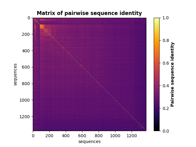
Compute the matrix of pairwise sequence identity

identity_matrix = c_msa.compute_seq_identity(sequences)

fig, ax = plt.subplots()
m = ax.imshow(identity_matrix, vmin=0, vmax=1, cmap='inferno')
ax.set_xlabel("sequences", fontsize=10)
ax.set_ylabel("sequences", fontsize=10)
ax.set_title('Matrix of pairwise sequence identity', fontweight="bold")
cb = fig.colorbar(m)
cb.set_label("Pairwise sequence identity", fontweight="bold")

Compute sequence weights

seq_weights, m_eff = c_pos.compute_seq_weights(sequences)
print('Number of effective sequences %d' %
      np.round(m_eff))

computing weight of seq 1/1376
computing weight of seq 101/1376
computing weight of seq 201/1376
computing weight of seq 301/1376
computing weight of seq 401/1376
computing weight of seq 501/1376
computing weight of seq 601/1376
computing weight of seq 701/1376
computing weight of seq 801/1376
computing weight of seq 901/1376
computing weight of seq 1001/1376
computing weight of seq 1101/1376
computing weight of seq 1201/1376
computing weight of seq 1301/1376
Number of effective sequences 1019

Compute conservation along the MSA

Di = c_pos.compute_conservation(sequences, seq_weights)

fig, ax = plt.subplots(figsize=(9, 4))
xvals = [i+1 for i in range(len(Di))]
xticks = [0, 50, 100, 150, 200, 250]
ax.bar(xvals, Di, color='k')
plt.tick_params(labelsize=11)
ax.set_xticks(xticks)
ax.set_xlabel('residues', fontsize=14)
ax.set_ylabel('Di', fontsize=14)

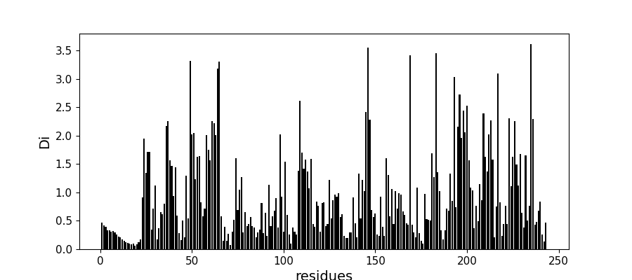
Text(72.97222222222221, 0.5, 'Di')

Compute the SCA coevolution matrix

SCA_matrix = c_pw.compute_sca_matrix(sequences, seq_weights)

fig, ax = plt.subplots()
im = ax.imshow(SCA_matrix, vmin=0, vmax=1.4, cmap='inferno')

ax.set_xlabel('residues', fontsize=10)
ax.set_ylabel(None)
ax.set_title('SCA matrix')
fig.colorbar(im, shrink=0.7)

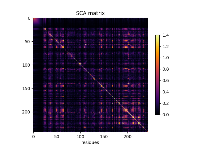
<matplotlib.colorbar.Colorbar object at 0x7f90ea6badd0>

Extraction of principal components (PCA analysis) and of independent components (ICA analysis) (this can take some time because of randomization) ————————————————-

n_components = 9
principal_components = c_deconv.extract_principal_components(
    SCA_matrix)
idpt_components = c_deconv.extract_independent_components(
    SCA_matrix,
    n_components=n_components)

Plot components

n_components_to_plot = n_components
if n_components_to_plot % 2:
    print('Odd number of components: the last one is discarded for \
          visualization')
    n_components_to_plot -= 1

pairs = [[x, x+1] for x in range(0, n_components_to_plot, 2)]
ncols = len(pairs)
plt.rcParams['figure.figsize'] = 14, 8
fig, axes = plt.subplots(nrows=2, ncols=len(pairs), tight_layout=True)
for k, [k1, k2] in enumerate(pairs):
    ax = axes[0, k]
    ax.plot(principal_components[k1], principal_components[k2], 'ok')
    ax.set_xlabel("PC %i" % (k1+1), fontsize=16)
    ax.set_ylabel("PC %i" % (k2+1), fontsize=16)

    ax = axes[1, k]
    ax.plot(idpt_components[k1], idpt_components[k2], 'ok')
    ax.set_xlabel("IC %i" % (k1+1), fontsize=16)
    ax.set_ylabel("IC %i" % (k2+1), fontsize=16)

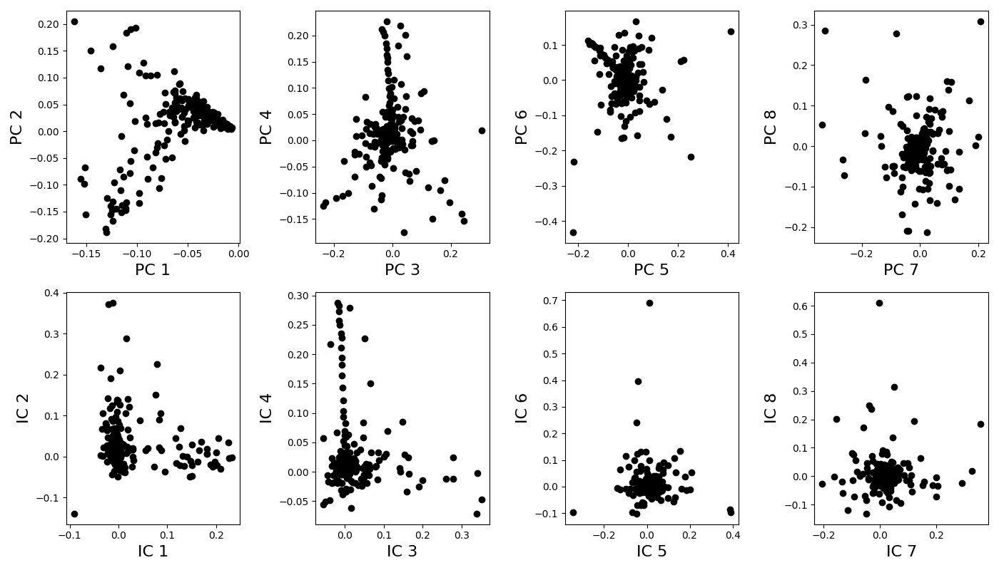
Odd number of components: the last one is discarded for           visualization

Extract sectors

sectors = c_deconv.extract_sectors(idpt_components, SCA_matrix)

print('Sector positions on (filtered) sequences:')
for isec, sec in enumerate(sectors):
    print('sector %d: %s' % (isec+1, sec))

Sector positions on (filtered) sequences:
sector 1: [64, 48, 145, 195, 63, 182, 199, 168, 146, 197, 144, 108, 222, 61, 196, 198, 194, 211, 49, 216, 208, 192, 234, 26, 35, 62, 235, 50, 155, 200, 23, 60, 76, 213, 73, 58, 114, 25]
sector 2: [140, 202, 52, 110, 78, 87, 81, 129, 75, 124, 33, 32, 128, 82, 207, 226, 120, 83, 69, 31]
sector 3: [225, 190, 212, 223, 180, 183, 184, 220, 224, 193, 172, 210, 142, 176, 160, 177, 217, 219, 161, 227]
sector 4: [0, 1, 2, 3, 4, 5, 6, 22, 7, 8, 9, 10, 11, 12, 13, 158, 14]
sector 5: [24, 228, 51, 215, 188]
sector 6: [97, 100, 98, 101, 95, 91, 107, 126, 102]
sector 7: [231, 109, 59, 53, 206, 131, 130]
sector 8: [57, 36, 111, 204, 34, 117]
sector 9: [46, 39, 37, 38, 156, 152, 41, 201, 149, 148, 143]

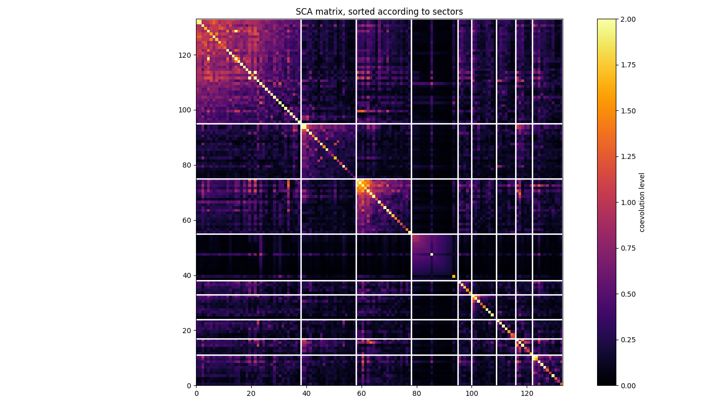
Plot coevolution within and between the sectors Each white square corresponds to a sector, with the residues ordered in decreasing contribution to the independent component associated from top to bottom and from left to right.

fig, ax = plt.subplots(tight_layout=True)

sector_sizes = [len(sec) for sec in sectors]
cumul_sizes = sum(sector_sizes)
sorted_pos = [s for sec in sectors for s in sec]

im = ax.imshow(SCA_matrix[np.ix_(sorted_pos, sorted_pos)],
               vmin=0, vmax=2,
               interpolation='none', aspect='equal',
               extent=[0, cumul_sizes, 0, cumul_sizes], cmap='inferno')
ax.set_title('SCA matrix, sorted according to sectors')
cb = fig.colorbar(im)
cb.set_label("coevolution level")

line_index = 0
for i in range(n_components):
    ax.plot([line_index + sector_sizes[i], line_index + sector_sizes[i]],
            [0, cumul_sizes], 'w', linewidth=2)
    ax.plot([0, cumul_sizes], [cumul_sizes - line_index,
                               cumul_sizes - line_index], 'w', linewidth=2)
    line_index += sector_sizes[i]

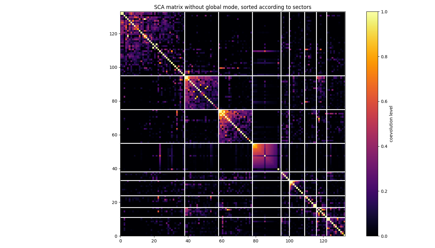
Do the same but for the SCA matrix where the global correlation mode has been removed and, hence, such that sectors are better highlighted. See Rivoire et al., PLOSCB, 2016

# removing global model (ngm = no global mode),
# i.e., removing first principal component
SCA_matrix_ngm = c_deconv.substract_first_principal_component(SCA_matrix)

# plotting
fig, ax = plt.subplots(tight_layout=True)
im = ax.imshow(SCA_matrix_ngm[np.ix_(sorted_pos, sorted_pos)], vmin=0, vmax=1,
               interpolation='none', aspect='equal',
               extent=[0, sum(sector_sizes), 0, sum(sector_sizes)],
               cmap='inferno')
ax.set_title('SCA matrix without global mode, sorted according to sectors')
cb = fig.colorbar(im)
cb.set_label("coevolution level")

line_index = 0
for i in range(n_components):
    ax.plot([line_index + sector_sizes[i], line_index + sector_sizes[i]],
            [0, sum(sector_sizes)], 'w', linewidth=2)
    ax.plot([0, sum(sector_sizes)], [sum(sector_sizes) - line_index,
                                     sum(sector_sizes) - line_index],
            'w', linewidth=2)
    line_index += sector_sizes[i]

Export sector sequences for all sequences as a fasta file The file can then be used for visualization along a phylogenetic tree as implemented in the cocoatree.visualization module

sector_1_pos = list(positions[sectors[0]])
sector_1 = []
for sequence in range(len(sequences_id)):
    seq = ''
    for pos in sector_1_pos:
        seq += loaded_seqs[sequence][pos]
    sector_1.append(seq)

c_io.export_fasta(sector_1, sequences_id, 'sector_1.fasta')

if False:  # need to be revised
    sector_1_pos = list(positions[sectors[0].items])
    sector_1 = []
    for sequence in range(len(sequences_id)):
        seq = ''
        for pos in sector_1_pos:
            seq += sequences[sequence][pos]
        sector_1.append(seq)

    c_io.export_fasta(sector_1, sequences_id, 'sector_1.fasta')

    # %
    # Export files necessary for Pymol visualization
    # Load PDB file of rat's trypsin
    pdb_seq, pdb_pos = c_io.load_pdb('data/3TGI.pdb', pdb_id='TRIPSIN',
                                     chain='E')
    # Map PDB positions on the MSA sequence corresponding to rat's trypsin:
    # seq_id='14719441'
    pdb_mapping = c_msa.map_to_pdb(pdb_seq, pdb_pos, sequences, sequences_id,
                                   ref_seq_id='14719441')
    # Export lists of the first sector positions and each residue's
    # contribution to the independent component to use for visualization on
    # Pymol.
    # The residues are ordered in the list by decreasing contribution score
    # (the first residue in the list is the highest contributing)
    c_io.export_sector_for_pymol(pdb_mapping, idpt_components.T, axis=0,
                                 sector_pos=sector_1_pos,
                                 ics=sectors,
                                 outpath='color_sector_1_pymol.npy')